Hello,
Firstly, thank you all for your time. I hope this problem is shared by the community and it is helpful for others too.
I am using pgrouting to asssess the centrality before and after the flooding in Rio Grande do Sul (Brazil). Calculating the centrality was easy using a origin destination matrix (OD) as Daniel Patterson mentioned in its post or Matthew Forrest or Regina O Obe in their books. However, increasing the size of the network or the number of origin and destination returned:
ERROR: invalid memory alloc request size 2450771848
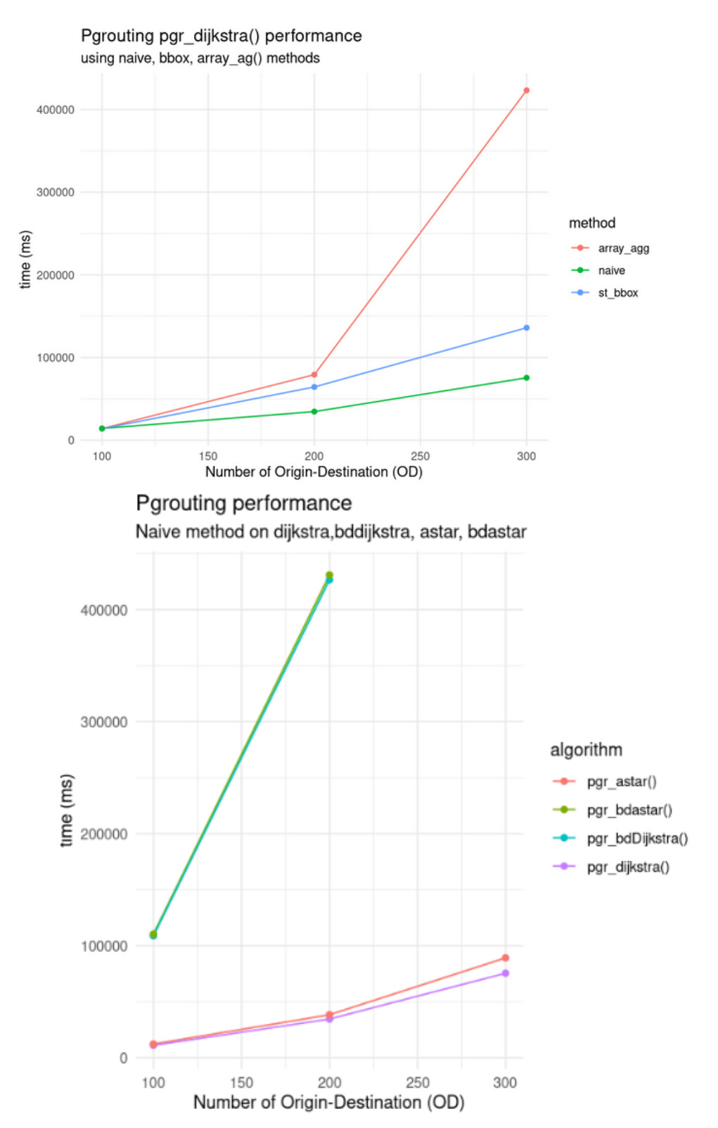
Apart from configuration tips (post), users reported different methods to optimize pgr_dijkstra. The “array_agg” method use the function array_agg() in the start vid and end vid parameters of pgr_dijkstra. The “st_bbox() method” only apply Dijkstra where a bounding box intersects with the start vid (origin) and end vid(destination), reducing rows. The simple or naive method uses an ARRAY() that constitutes the OD-matrix, where the LEFT JOIN added the geometry from the original network table using the ID.
---simple or naive approach
SELECT
     b.id,
     b.the_geom,
     count(the_geom) as centrality
FROM
      pgr_dijkstra(
        'SELECT
	        id,
	        source,
	        target,
	        cost
      	FROM
        	porto_alegre_net_largest',
            ARRAY(SELECT net_id AS start_id FROM weight_sampling_100_origin) ,
            ARRAY(SELECT net_id AS end_id FROM weight_sampling_100_origin ),
            directed := TRUE) j
     LEFT JOIN porto_alegre_net_largest AS b
       ON j.edge = b.id
     GROUP BY
       b.id,
       b.the_geom
  ORDER BY
       centrality DESC;
I expected to obtain less computing costs using bbox or array_agg(), however, these are the preliminary performance results. The simple way using pgr_dijkstra() and an array for origin and destination achieved a better performance returning the results in less time.
Then, I used this naive method using different algorithms. I expected pgr_astar() to be faster than pgr_dijkstra(), since pgr_astar() does not explore each segment of the network, unlike pgr_dijkstra that explores all the network. The results obtained indicated that it is again pgr_dijkstra() the algorith that required less time to return the results.
This is the google drive link to the data to reproduce the results. These are the files:
- network folder: it contains “porto_alegre_net_largest.geojson”, which represents the network before the flooding of the study area, and its respective vertice table “porto_alegre_net_largest_vertices_pgr.geojson”. There are similar tables to run pgr_astar().
- origin_destination_matrix: it contains “weight_sampling_100_origin.geojson” & “weight_sampling_100_destination.geojson”, which represent the origin and destination points. There are similar tables for 200, 300 and 500. 500 points is my current limit that I can not run.
- metrics_algorithm_naive_osgeo.csv: csv that contains “metrics_algorithm_naive_osgeo.csv” & “metrics_and_quries_method_dijkstra_osgeo.csv” the query used, it’s performance (explain analyze) method or algorithm.
Thank you very much for your time and attention! Your help would be very valuable to improve the analysis that aims to identify the most central roads.
Images from the flooding by global-flood.emergency.copernicus